Try balancing a broomstick on your palm. Your brain is constantly making tiny corrections; left, right, a tiny flick of the wrist. Now imagine writing software to do the same thing, swing a hanging pole up to vertical and hold it there turns out to be a clean problem for comparing two very different control philosophies on identical terms.
This is the cart-pole swing-up task: a pole starts hanging straight down, and the controller must inject energy to raise it, bring it to the upright position, and keep it there against gravity. In Part 1, I compared Model Predictive Control (MPC) and Reinforcement Learning (RL) conceptually. This post is the implementation: I walk through every design decision in both controllers and report results from running them on the same simulator.
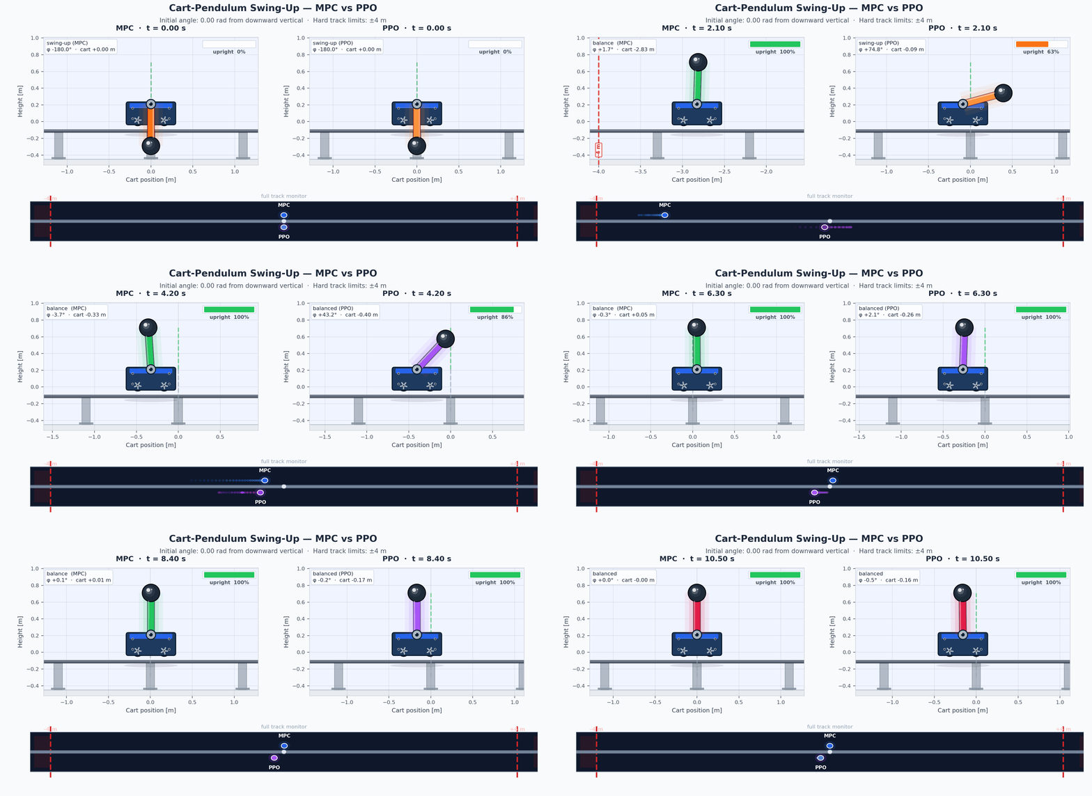
1. The System and the Task
Before choosing a controller, the problem has to be defined precisely.
State and input
A cart of mass $M$ slides along a horizontal rail. A rigid rod of mass $m$ is pinned to the top of the cart and swings freely in the vertical plane. The only actuator is a horizontal force $u$ applied to the cart.
State vector and convention
$$\mathbf{s} = \begin{bmatrix} p \\ \dot{p} \\ \theta \\ \dot{\theta} \end{bmatrix} \in \mathbb{R}^4, \qquad u \in [-15,\ 15]\;\text{N}$$$p$ = cart position (m), $\theta$ = pole angle from the downward vertical. Hanging down is $\theta = 0$, upright is $\theta = \pi$. The error from upright is
$$\phi = \operatorname{wrap}(\theta - \pi) \in [-\pi, \pi).$$The physical parameters:
| Symbol | Quantity | Value |
|---|---|---|
| $M$ | cart mass | $1.0\;\text{kg}$ |
| $m$ | pole mass | $0.3\;\text{kg}$ |
| $l$ | pole half-length (pivot to centre of mass) | $0.5\;\text{m}$ |
| $g$ | gravity | $9.81\;\text{m/s}^2$ |
| $\Delta t$ | time step | $0.05\;\text{s}$ |
What counts as success
I define success strictly: the pole must be sustained in the upright region during the final second, and the cart must stay on the track:
$$|\phi_t| \lt 0.05\;\text{rad} \quad \forall\, t \in [T-1,\, T], \qquad |p_t| \le 4\;\text{m}\;\; \forall\, t.$$Counting a single crossing of $\theta = \pi$ as "success" would reward a controller that flings the pole through vertical and lets it fall back. That is not balance. Requiring a held one-second window (20 steps at $\Delta t = 0.05\;\text{s}$) eliminates those false positives.
2. Simulating the Physics
Both controllers interact with the same nonlinear simulator. If the simulator is wrong, both controllers are evaluated on a broken problem, so this is worth getting exactly right.
Equations of motion
The dynamics follow from Lagrangian mechanics. I use the generalized coordinates $(p, \theta)$ but write the trigonometry in the upright-error angle $\theta_u = \theta - \pi$, because that is the coordinate both the plant and the controllers actually evaluate. With the pole modelled as a uniform rod, its centre of mass sits a distance $l$ from the pivot at
$$x_c = p + l\sin\theta_u, \qquad y_c = l\cos\theta_u,$$so $\dot{x}_c = \dot{p} + l\dot{\theta}\cos\theta_u$ and $\dot{y}_c = -l\dot{\theta}\sin\theta_u$.
Kinetic and potential energy
The cart contributes $\tfrac{1}{2}M\dot{p}^2$; the pole contributes its translational energy $\tfrac{1}{2}m(\dot{x}_c^2 + \dot{y}_c^2)$ plus the rotation of the rod about its own centre of mass, $\tfrac{1}{2}I_{\mathrm{cm}}\dot{\theta}^2$ with $I_{\mathrm{cm}} = \tfrac{1}{3}ml^2$. Collecting terms:
$$T = \tfrac{1}{2}(M+m)\dot{p}^2 + ml\,\dot{p}\,\dot{\theta}\cos\theta_u + \tfrac{1}{2}\underbrace{\bigl(\tfrac{1}{3}ml^2 + ml^2\bigr)}_{I\,=\,\frac{4}{3}ml^2}\dot{\theta}^2, \qquad V = mgl\cos\theta_u.$$The $\tfrac{4}{3}ml^2$ is the rod's moment of inertia about the pivot - the parallel-axis sum of $I_{\mathrm{cm}} = \tfrac{1}{3}ml^2$ and $ml^2$ - and is the signature of the uniform-rod model. A point mass on a massless rod would give only $ml^2$.
Applying the Euler–Lagrange equations with the generalized force $u$ on $p$ and none on $\theta$ gives two coupled equations:
$$\begin{align} (M+m)\,\ddot{p} + ml\,\ddot{\theta}\cos\theta_u - ml\,\dot{\theta}^2\sin\theta_u &= u, \tag{1}\\[4pt] \tfrac{4}{3}ml^2\,\ddot{\theta} + ml\,\ddot{p}\cos\theta_u - mgl\sin\theta_u &= 0. \tag{2} \end{align}$$These are linear in the accelerations $(\ddot{p}, \ddot{\theta})$. Solving for $\ddot{p}$ from (1) and back-substituting into (2) yields the explicit form the simulator integrates:
$$\ddot{\theta} = \frac{g\sin\theta_u - \cos\theta_u \cdot \tau}{ l\!\left(\dfrac{4}{3} - \dfrac{m\cos^2\!\theta_u}{M+m}\right) }, \tag{3}$$ $$\ddot{p} = \tau - \frac{ml\,\ddot{\theta}\cos\theta_u}{M+m}, \tag{4}$$where
$$\tau = \frac{u + ml\,\dot{\theta}^2\sin\theta_u}{M+m}$$is the effective cart acceleration before accounting for inertial coupling with the pole. The $\cos^2\theta_u$ term in the denominator of (3) is exactly the inertial coupling: the cart's reaction reduces the pole's effective inertia by an amount that depends on the pole's angle.
Sign convention
At the upright equilibrium $\theta_u = 0$, so $\cos\theta_u = 1$ and the denominator is positive. The $g\sin\theta_u$ term in $\ddot{\theta}$ is destabilising ; a small tilt grows, which is the defining property of the inverted equilibrium. Throughout, $\theta$ is measured from the downward vertical; the controllers operate in the error coordinate $\phi = \theta - \pi$. The positive rotational direction is fixed by the equations above: the pole tip sits at $x_{\text{tip}} \approx p + l\phi$ near upright, so a positive force gives $\ddot{\phi} \lt 0$ at upright; the pole tips back against the push, exactly as a physical cart-pole does.
Integration: RK4
The simulator advances the state with fourth-order Runge–Kutta rather than forward Euler. Euler is simple but not accurate enough at $\Delta t = 0.05\;\text{s}$ for a stiff, unstable system:
$$\begin{align} k_1 &= f(\mathbf{s}_k,\, u_k), & k_2 &= f\!\left(\mathbf{s}_k + \tfrac{\Delta t}{2}k_1,\, u_k\right),\\[2pt] k_3 &= f\!\left(\mathbf{s}_k + \tfrac{\Delta t}{2}k_2,\, u_k\right), & k_4 &= f(\mathbf{s}_k + \Delta t\, k_3,\, u_k),\\[4pt] \mathbf{s}_{k+1} &= \mathbf{s}_k + \frac{\Delta t}{6}(k_1 + 2k_2 + 2k_3 + k_4). \end{align}$$RK4 has local truncation error $O(\Delta t^5)$ per step and global error $O(\Delta t^4)$, versus Euler's $O(\Delta t^2)$ local and $O(\Delta t)$ global. Both controllers run on this same integrator, so any performance gap reflects the controllers, not the physics.
3. The Reward: A Single Shared Objective
I wanted one scoring function usable for both PPO training and post-hoc comparison. Using different objectives for each would make the comparison meaningless.
The difficulty is that a naive "reward only when upright" signal is silent during the entire swing-up. The reward needs to be dense.
Energy as a shaping signal
Even when the pole is far from upright, we know how much mechanical energy it needs to get there. Taking the downward rest position as the zero of potential energy, and using the same uniform-rod model as the plant ($I = \tfrac{4}{3}ml^2$ about the pivot), the pole's mechanical energy is
$$E(\mathbf{s}) = \tfrac{1}{2}I\dot{\theta}^2 + mgl(1-\cos\theta) = \tfrac{2}{3}ml^2\dot{\theta}^2 + mgl(1-\cos\theta),$$and the energy at the upright equilibrium $(\theta = \pi,\; \dot{\theta} = 0)$ is
$$E_{\mathrm{target}} = mgl(1-\cos\pi) = 2mgl.$$The kinetic term uses the rod's rotational inertia, not the point-mass form $\tfrac{1}{2}m(l\dot{\theta})^2$, which would undercount the rotational energy by a factor of $\tfrac{4}{3}$. Keeping the energy model consistent with the integrated dynamics is what makes "$E = E_{\mathrm{target}}$" mean exactly what it says: the pole has just enough energy to coast to upright; the property the swing-up logic relies on.
The shared reward function
Shared reward $r(\mathbf{s}, u)$; used by both MPC and PPO
$$r(\mathbf{s}, u) = \underbrace{(1 + \cos\phi)}_{\substack{\text{upright score}\\\in[0,2]}} + 0.75\min\!\left(\frac{E}{E_{\mathrm{target}}},\;1\right) - 0.005\,u^2 - 0.05\,\dot{\theta}^2 - 0.20\,p^2 - 0.03\,\dot{p}^2.$$Each term has a clear job:
- $1+\cos\phi$: smooth signal that peaks at 2 (upright) and bottoms at 0 (hanging), avoiding the discontinuity of an indicator function.
- Energy bonus: positive reward during swing-up, not just at the goal. Saturates at 0.75 once $E \ge E_{\mathrm{target}}$ so the agent is not rewarded for excess kinetic energy.
- Force penalty: discourages wasteful bang-bang control.
- Angular-velocity penalty: damps spinning during balance.
- Position and cart-velocity penalties: make cart regulation an explicit objective, so the policy parks the cart at the centre and brings it to rest rather than balancing the pole wherever the cart drifts. The position coefficient is worth tuning empirically: at $0.12$ the trained policy balanced perfectly but parked the cart $0.4$ m off-centre indefinitely; the centering gradient was below what training resolves. At $0.20$ it parks within about $0.2$ m - the offset shrinks with the coefficient, a knob to set empirically, not by feel.
Termination is part of the objective
One guard lives in the training environment rather than the reward formula: leaving the $\pm 4$ m track terminates the episode with a $-100$ penalty. Without it, termination is free - an agent stuck in a low-reward state (hanging, far off-centre) could profit from driving off the track to stop the negative reward stream. If any reachable state has negative reward, an unpenalized exit is an escape hatch the optimizer will eventually find.
4. The MPC Controller
The MPC controller is hybrid: an energy-shaping law performs the swing-up, and a receding-horizon quadratic program (QP) takes over once the pole is near upright. The interesting engineering is in the handoff.
Linearising around upright
Near $\phi = 0$ the nonlinear dynamics are approximately linear. I define the MPC error state $\mathbf{x} = \begin{bmatrix} p & \dot{p} & \phi & \dot{\theta} \end{bmatrix}^T$ and linearise equations (3)–(4) around $(\mathbf{x}, u) = (\mathbf{0}, 0)$:
$$\dot{\mathbf{x}} = \mathbf{A}_c \mathbf{x} + \mathbf{B}_c u,$$ $$\mathbf{A}_c = \begin{bmatrix} 0 & 1 & 0 & 0 \\ 0 & 0 & -\tfrac{mlg}{(M+m)\,d} & 0 \\ 0 & 0 & 0 & 1 \\ 0 & 0 & \tfrac{g}{d} & 0 \end{bmatrix}, \qquad \mathbf{B}_c = \begin{bmatrix} 0 \\ \tfrac{1}{M+m} - \tfrac{ml\,f_\alpha}{M+m} \\ 0 \\ f_\alpha \end{bmatrix},$$where $d = l\bigl(\tfrac{4}{3} - \tfrac{m}{M+m}\bigr)$ and $f_\alpha = -\tfrac{1}{(M+m)d}$.
The entry $g/d$ in the $\dot{\theta}$ row is the instability made explicit: with our parameters it gives an open-loop unstable eigenvalue of $\sqrt{g/d} \approx 4.2\;\text{s}^{-1}$, so any nonzero $\phi$ grows exponentially without control.
Discretising the model
The MPC prediction model must be discrete-time, and the discretisation matters more than it looks. The Euler approximation $\mathbf{A}_d = \mathbf{I} + \Delta t \mathbf{A}_c$ is fine for small $\Delta t$, but here it is meaningfully off: with the unstable mode at $\lambda \approx 4.2\;\text{s}^{-1}$, Euler's one-step growth factor is $1 + \lambda\Delta t = 1.211$ against an exact $e^{\lambda\Delta t} = 1.235$ - about a 2% error per step in the dominant mode, enough to bias the optimisation toward a model that drifts from the plant.
The model therefore uses zero-order-hold (ZOH) discretisation, which is exact for piecewise-constant inputs:
ZOH discretisation - exact for constant-input intervals
$$\begin{bmatrix} \mathbf{A}_d & \mathbf{B}_d \\ \mathbf{0} & \mathbf{I} \end{bmatrix} = \exp\!\left( \begin{bmatrix} \mathbf{A}_c & \mathbf{B}_c \\ \mathbf{0} & \mathbf{0} \end{bmatrix} \Delta t \right)$$Computed once at startup with scipy.linalg.expm. Under ZOH, $\mathbf{x}_{k+1} = \mathbf{A}_d \mathbf{x}_k + \mathbf{B}_d u_k$ is the exact solution of the continuous-time ODE for any constant $u_k$, regardless of step size.
The terminal cost has a principled value
A finite-horizon MPC with horizon $N$ approximates the true infinite-horizon problem. The bias from truncating the horizon can be removed by setting the terminal cost matrix $\mathbf{P}$ to the optimal infinite-horizon cost-to-go of the unconstrained linear-quadratic problem. With that choice, the receding-horizon controller inherits the stability of the underlying LQR. This $\mathbf{P}$ is the unique positive-definite solution of the discrete algebraic Riccati equation (DARE):
$$\mathbf{P} = \mathbf{Q} + \mathbf{A}_d^T \mathbf{P} \mathbf{A}_d - \mathbf{A}_d^T \mathbf{P} \mathbf{B}_d \!\left(\mathbf{R} + \mathbf{B}_d^T \mathbf{P} \mathbf{B}_d\right)^{-1} \mathbf{B}_d^T \mathbf{P} \mathbf{A}_d, \tag{5}$$
computed once with scipy.linalg.solve_discrete_are.
A hand-picked multiple $c\mathbf{Q}$ carries no stability guarantee and is strictly worse for
the same compute.
The optimisation solved each step
Every 50 ms the controller solves:
MPC QP - solved at each time step
$$\min_{\mathbf{u}_{0:N-1}} \sum_{t=1}^{N-1} \mathbf{x}_{t}^T \mathbf{Q}\, \mathbf{x}_{t} + \sum_{t=0}^{N-1} u_t \mathbf{R}\, u_t + \mathbf{x}_N^T \mathbf{P}\, \mathbf{x}_N$$subject to $\mathbf{x}_{t+1} = \mathbf{A}_d \mathbf{x}_t + \mathbf{B}_d u_t$, $\quad |u_t| \le 15\;\text{N}$, $\quad \mathbf{x}_0 = \hat{\mathbf{x}}_k$ (current error state).
The tuning settled on:
$$N = 40\;\text{steps (2 s lookahead)},\quad \mathbf{Q} = \operatorname{diag}(2,\; 0.5,\; 80,\; 2),\quad \mathbf{R} = 0.05.$$
The large $Q_{33} = 80$ makes angle the dominant cost. The asymmetry between $Q_{11}=2$ (position)
and $Q_{22}=0.5$ (velocity) lets the cart drift gently but penalises fast excursions. Only $u_0^*$
from the optimal sequence is applied. The problem is built once with a cp.Parameter
for the initial state and solved each step with warm_start=True, which avoids
re-canonicalization.
# Built once at __init__
self._x0 = cp.Parameter(4)
x = cp.Variable((4, N + 1))
u = cp.Variable((1, N))
cost = sum(cp.quad_form(x[:, t], Q) for t in range(1, N))  # x_1..x_{N-1}
cost += sum(cp.quad_form(u[:, t], R) for t in range(N))
cost += cp.quad_form(x[:, N], P)   # terminal state: DARE P alone

self._problem = cp.Problem(cp.Minimize(cost), constraints)

# Called every step — fast because the problem is already built
self._x0.value = error_state
self._problem.solve(solver=cp.CLARABEL, warm_start=True)
Swing-up by energy shaping
The linear MPC is only valid near upright ($|\phi| \lesssim 0.35\;\text{rad}$). To get there from hanging I use an energy-shaping controller. The form falls out of asking how the cart's motion changes the pole's energy.
Treat the pole's mechanical energy about the pivot and recall from the pole equation (2) that the angular acceleration driven by a cart acceleration $\ddot{p}$ obeys $I\ddot{\theta} = -mgl\sin\theta + ml\,\ddot{p}\cos\theta$. Differentiating $E$ along the trajectory, the gravity terms cancel and only the cart-coupling survives:
Energy rate - why the law has the form it does
$$\dot{E} = \dot{\theta}\bigl(I\ddot{\theta} + mgl\sin\theta\bigr) = ml\,\ddot{p}\,\bigl(\dot{\theta}\cos\theta\bigr).$$The cart can only inject energy through the product $\dot{\theta}\cos\theta$.
Taking the Lyapunov candidate $\mathcal{V} = \tfrac{1}{2}(E - E_{\mathrm{target}})^2$ and commanding $\ddot{p} \propto \operatorname{sign}(E_{\mathrm{target}} - E)\,\dot{\theta}\cos\theta$ gives
$$\dot{\mathcal{V}} = (E - E_{\mathrm{target}})\,\dot{E} \;\propto\; -|E - E_{\mathrm{target}}|(\dot{\theta}\cos\theta)^2 \le 0,$$so $E$ is driven monotonically toward $E_{\mathrm{target}}$. The control law is simply
$$u_E = k_E\,\dot{\theta}\cos\theta, \qquad k_E = 28,$$with the sign flipped once $E \ge E_{\mathrm{target}}$ to switch from pumping energy in to bleeding it off.
The startup problem. At rest, $(\theta, \dot{\theta}) = (0, 0)$ gives $u_E = 0$ - the system sits at the stable downward equilibrium and never moves. I break the symmetry with a small kick toward the centre:
$$\text{if } |u_E| \lt 0.2 \text{ and } E \lt 0.05\,E_{\mathrm{target}}: \quad u \leftarrow \operatorname{sign}(-p)\cdot 3\;\text{N}.$$Cart drift. Left alone the cart wanders toward the boundaries during swing-up, so I add linear centering terms:
$$u_{\mathrm{swing}} = \operatorname{clip}\!\left(u_E - 1.2\,p - 2.0\,\dot{p},\; -15,\; 15\right).$$Switching modes without chattering
The controller switches from swing-up to linear MPC when
$$|\phi| \le 0.35\;\text{rad} \quad\text{and}\quad E \le 1.08\,E_{\mathrm{target}}.$$The energy condition matters: a pole with too much kinetic energy will overshoot upright even with zero force, and the linear controller would fight it. It exits back to swing-up only when $|\phi| \gt 0.60\;\text{rad}$. The wider exit threshold creates hysteresis around the boundary - without it the controller would oscillate between modes many times per second.
5. The PPO Agent
The RL approach uses none of the math above. It observes the state, takes actions, and receives the shared reward. The questions are what it must learn and how to set up training so it actually learns it.
Observation design
The policy network receives a 5-dimensional observation:
$$\mathbf{o}_t = \begin{bmatrix} p_t & \dot{p}_t & \cos\theta_t & \sin\theta_t & \dot{\theta}_t \end{bmatrix}^T.$$The angle is encoded as $(\cos\theta, \sin\theta)$ rather than the raw $\theta$. At $\theta = \pm\pi$ the raw angle wraps - it jumps by $2\pi$ - so to the network a smooth physical transition looks like an enormous discontinuity. The trigonometric encoding is continuous everywhere. The bounds for $(\cos\theta, \sin\theta)$ are declared as $[-1, 1]$, not infinity, so the running normalizer treats them as the bounded quantities they are.
Observation normalisation
The five components have very different scales: position lives in roughly $[-4, 4]$, while angular velocity during a fast spin can reach $\pm 20\;\text{rad/s}$. Without normalisation, gradients from the high-variance dimensions dominate. I apply a running mean–variance normaliser:
$$\tilde{o}_i = \operatorname{clip}\!\left( \frac{o_i - \mu_i}{\sqrt{\sigma_i^2 + \varepsilon}},\; -10,\; 10 \right),$$with $\mu_i$ and $\sigma_i^2$ updated online during training and saved alongside the model. At inference the same frozen statistics are applied, so there is no train/eval distribution shift.
The PPO update rule
PPO learns a Gaussian policy $\pi_\psi(a|\mathbf{o})$ by maximising a clipped surrogate objective. With the probability ratio $\rho_t = \pi_\psi(a_t|\mathbf{o}_t) / \pi_{\psi_{\mathrm{old}}}(a_t|\mathbf{o}_t)$:
PPO clipped objective
$$\mathcal{L}^{\mathrm{CLIP}}(\psi) = \mathbb{E}_t\!\Bigl[ \min\!\Bigl( \rho_t\,\hat{A}_t,\;\; \operatorname{clip}(\rho_t,\, 1-\varepsilon,\, 1+\varepsilon)\,\hat{A}_t \Bigr) \Bigr], \quad \varepsilon = 0.2.$$The clip is the central idea: no single update can move the policy by more than $\varepsilon$ in probability-ratio terms, which prevents the catastrophic collapse that plagues vanilla policy gradient. The advantage $\hat{A}_t$ is estimated with GAE ($\lambda = 0.95$):
$$\delta_t = r_t + \gamma V_\phi(\mathbf{o}_{t+1}) - V_\phi(\mathbf{o}_t), \qquad \hat{A}_t = \sum_{l=0}^{\infty}(\gamma\lambda)^l\,\delta_{t+l}.$$$\lambda = 0.95$ interpolates between high-variance Monte Carlo ($\lambda=1$) and biased TD(0) ($\lambda=0$).
Curriculum over initial states
I use a mixed start distribution:
$$\theta_0 \sim \begin{cases} \mathcal{U}(\pi - 0.25,\; \pi + 0.25) & \text{prob. } 0.35 \quad\text{(near upright)} \\ \mathcal{U}(-0.15,\; 0.15) & \text{prob. } 0.65 \quad\text{(near hanging)} \end{cases}$$with randomised velocities $\dot{p}_0 \sim \mathcal{U}(-0.5, 0.5)$, $\dot{\theta}_0 \sim \mathcal{U}(-1.0, 1.0)$. The velocity randomisation forces the policy to handle near-balance states with nonzero momentum - exactly the condition it faces immediately after a real swing-up.
Training configuration
| Hyperparameter | Value |
|---|---|
| Total timesteps | $1\,000\,000$ |
| Vectorised environments | 4 |
| Rollout steps per env | 1024 |
| Minibatch size | 256 |
| PPO epochs per rollout | 10 |
| Discount $\gamma$ | 0.99 |
| GAE $\lambda$ | 0.95 |
| Clip $\varepsilon$ | 0.2 |
| Entropy coefficient $c_2$ | 0.01 |
| Learning rate | $3\times 10^{-4}$, linear decay |
| Network | two 128-unit hidden layers |
| Obs normalisation | running mean/var, clip $= 10$ |
6. Results
Both controllers achieve sustained balance on all five tested starting angles. To compare them on equal footing I score each trajectory by its cumulative shared reward - the same objective PPO trains on - over a 10 s rollout (higher is better), and report total control effort $\sum_k u_k^2$, the widest cart excursion, and the time $t_{\mathrm{up}}$ at which the pole first enters the $\pm 0.05\;\text{rad}$ upright window.
| $\theta_0$ | MPC | PPO | MPC return | PPO return | MPC $\sum u^2$ | PPO $\sum u^2$ | max $|p|$ (MPC / PPO) | $t_{\mathrm{up}}$ (MPC / PPO) |
|---|---|---|---|---|---|---|---|---|
| 0.00 rad | ✓ | ✓ | 341.9 | 356.5 | 6922 | 1540 | 3.27 m / 1.12 m | 2.1 s / 3.1 s |
| 0.05 rad | ✓ | ✓ | 346.5 | 355.1 | 7247 | 1535 | 3.27 m / 1.11 m | 2.2 s / 3.0 s |
| 0.10 rad | ✓ | ✓ | 289.3 | 354.2 | 7909 | 1500 | 3.79 m / 1.09 m | 2.1 s / 3.0 s |
| 0.15 rad | ✓ | ✓ | 280.6 | 353.4 | 8357 | 1470 | 3.77 m / 1.08 m | 2.3 s / 3.0 s |
| 0.20 rad | ✓ | ✓ | 443.3 | 352.7 | 5818 | 1439 | 2.69 m / 1.06 m | 1.5 s / 3.0 s |
Three things stand out:
- PPO wins the shared reward on four of five angles - the penalty bill, not swing-up speed, decides it. MPC still reaches the upright window first (1.5–2.3 s versus a remarkably consistent ${\sim}3$ s for the policy), and every extra second of swing-up costs roughly 50 reward. But MPC's wide excursions cost more than its speed buys back: at $\theta_0 = 0.10$–$0.15$ it loses ${\approx}120$ reward to the position penalty alone, while PPO's entire penalty bill is ${\approx}15$. The exception is $\theta_0 = 0.20$, where MPC's fastest swing-up (1.5 s, with its smallest excursion) posts the best score in the whole table.
- PPO is dramatically gentler. It uses four-to-six times less control effort and swings up within $\approx 1.1\;\text{m}$ of centre, while MPC flings the cart out to $\approx 2.7$–$3.8\;\text{m}$. If actuator wear, energy budget, or track length mattered, PPO would be the clear choice.
- Both park the cart once balanced, MPC more precisely. Over the final two seconds MPC holds the cart within about a centimetre of the origin; PPO settles about twenty centimetres off-centre and stays there - the residual offset of a learned policy whose centering gradient flattens near the origin, where a deterministic LQR-style balance drives the error to zero.
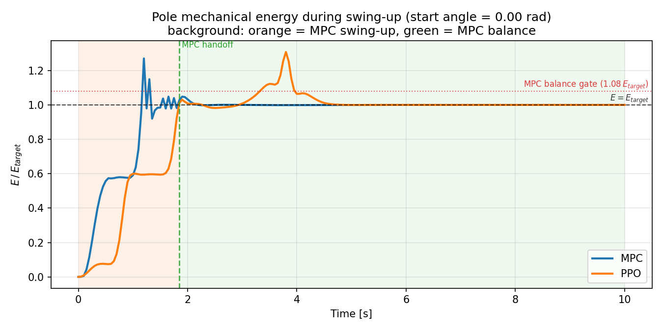
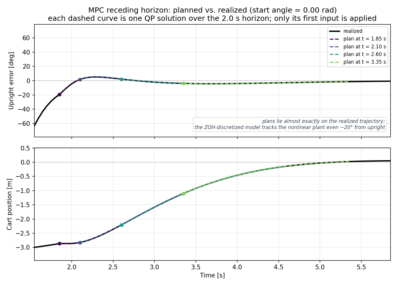
Qualitative differences:
- MPC's swing-up is structured and legible. The energy controller produces clean pumping oscillations, then hands off to the QP; the balance phase is smooth, with small precise corrections.
- PPO uses one continuous policy. There is no explicit mode switch - the same network does both swing-up and balance, and in the animation you cannot see a "switchover."
- Compute per step. PPO inference is ${\sim}0.06\;\text{ms}$ (one forward pass). An MPC balance solve is ${\sim}2.3\;\text{ms}$ (CLARABEL, $N=40$) - roughly forty times slower per step, but both are comfortably real-time at a 50 ms control period.
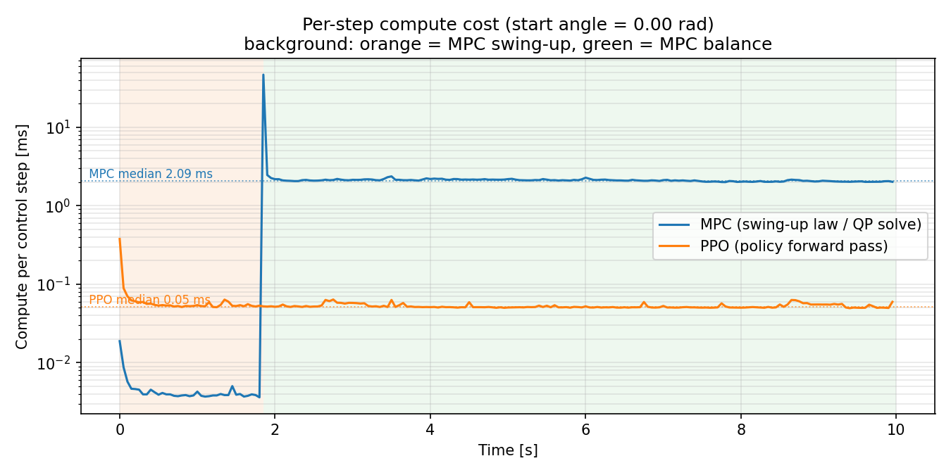
7. Practical Takeaways
A few design choices did most of the work in getting both controllers to behave.
Discretise the MPC model exactly
A linear MPC's quality is capped by the fidelity of its prediction model. ZOH
(scipy.linalg.expm) is exact for piecewise-constant inputs at any $\Delta t$ and
costs one matrix exponential at startup; an Euler model solves identically but optimises a
plant that quietly drifts.
Use the DARE terminal cost
Setting the terminal weight $\mathbf{P}$ to the infinite-horizon cost-to-go (one call to
solve_discrete_are) is what turns a finite-horizon QP into a controller with an
LQR stability guarantee. A hand-picked multiple of $\mathbf{Q}$ has no such guarantee and is
strictly worse for the same compute.
Shape the reward, and bound it
Reward design is RL's counterpart to tuning $\mathbf{Q}$ and $\mathbf{R}$. A pure angle reward is degenerate here - spinning the pole accrues reward through angular velocity without ever stabilising - which is exactly why the energy bonus saturates at $E_{\mathrm{target}}$ instead of rewarding raw energy.
Define success as sustained balance, not a crossing
A pole passing through $\phi = 0$ at $\dot{\theta} = 8\;\text{rad/s}$ is not balanced. Requiring a held one-second window removes a large class of lucky-looking single-step "successes."
Get the observation representation right
The $(\cos\theta, \sin\theta)$ encoding converges faster and yields a more robust policy than raw $\theta$, which is discontinuous at the wrap boundary. The two-layer, 128-unit network was never the bottleneck - representation mattered more than capacity.
Keep the energy model consistent with the plant
The swing-up law and the reward both read a mechanical-energy value, so that value must match the uniform-rod dynamics the simulator integrates (rotational inertia included). When a quantity feeds a threshold or a reward rather than just a plot, "approximately right" silently degrades behaviour - a zero-force conservation check is a cheap way to confirm it.
8. When Would I Reach for Each?
| MPC | PPO | |
|---|---|---|
| Needs a dynamics model | Yes (linearised) | No |
| Training time | None | ~1M steps |
| Hard constraints | Explicit in the QP | Clipping only |
| Swing-up strategy | Hand-crafted | Learned from reward |
| Stability certificate | Yes (via DARE/LQR) | No formal guarantee |
| Interpretability | High | Low (opaque weights) |
| Compute per step | ~2.3 ms (balance QP) | ~0.06 ms |
| Control effort (this task) | High | 4–6× lower |
| Main design effort | Linearisation, $\mathbf{Q}/\mathbf{R}$, mode logic | Reward, curriculum, normalisation |
| Failure mode | Model mismatch, mode chatter | Reward hacking, training instability |
The takeaway after building both: the design effort is comparable; it just lives in a different place. MPC demands correct math (linearisation, ZOH, DARE) and careful mode switching. RL demands a dense, well-shaped reward, sound observation design, and enough training to discover both behaviours. On this problem the trained policy posts the higher shared reward on four of five angles: MPC still reaches upright about a second sooner, but under the shared objective its wide cart excursions cost more than the speed buys back. MPC keeps the stability certificate, explicit constraint handling, and centimetre-precise parking; the policy counters with four-to-six times less actuation, a third of the track usage, and a per-step cost forty times lower - a genuinely different trade-off rather than a strictly weaker one.
I would reach for MPC when I have a reliable model and need hard constraint satisfaction with a stability guarantee. I would reach for RL when the dynamics are complex, uncertain, or multi-modal in ways that are awkward to capture in a QP.
9. Code
The code is available here. If you see bugs or any gaps, open an issue on GitHub.
References
- Schulman et al. (2017). Proximal Policy Optimization Algorithms. arXiv:1707.06347.
- Schulman et al. (2015). High-Dimensional Continuous Control Using Generalised Advantage Estimation. arXiv:1506.02438.
- Rawlings, Mayne & Diehl (2017). Model Predictive Control: Theory, Computation, and Design. Nob Hill Publishing.
- Raffin et al. (2021). Stable-Baselines3. JMLR 22(268).
- Diamond & Boyd (2016). CVXPY: A Python-Embedded Modeling Language for Convex Optimization. JMLR 17(83).
- Part 1: Reinforcement Learning vs Model Predictive Control.