The second policy I trained had just outperformed my hand-written controller in simulation, on courses it had never seen, at twice the speed. On the real car it saturated its steering within two seconds, oscillated between full left and full right, and lost the line. Six versions later, a policy trained entirely in simulation drove the real track from start to finish without any fine-tuning. Almost nothing that made the difference was a change to the learning algorithm. It was a sequence of measurements that showed, one by one, where the simulator disagreed with the car.
This article follows that sequence. It covers how I identified the vehicle using only the sensors already on it, how the simulator models the motors, the sensors and the communication link, how the policy is trained with PPO and an asymmetric critic, and how I validated the simulator by asking it to predict failures that had already happened on the floor. It closes with the gap that remains, measured from a phone video, and a short control-theoretic explanation of why it produces exactly the oscillation the camera recorded.
It continues the series that compared reinforcement learning and model predictive control on paper in Part 1 and on a simulated cart-pole in Part 2.
The platform and the problem
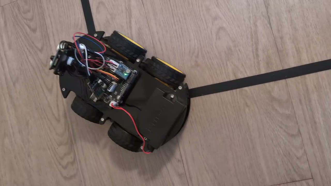
The Elegoo V4 is a four-wheel skid-steer car built around an Arduino UNO, a TB6612FNG motor driver and four TT gear motors. Its only line sensing is three analog IR reflectance sensors spaced 15 mm apart, and its only range sensing is an HC-SR04 ultrasonic sensor on a front servo. It has no wheel encoders and no IMU. The controller runs on a laptop and communicates with the Arduino through a BLE UART module at roughly 18.6 Hz. The test track is 15 mm black tape on light laminate: a 1.5 m straight, a sharp 90° right turn and a 1.2 m second leg.
Formally, this is a partially observed control problem with uncertain dynamics. The state $s_t$ contains the car's pose and velocities, the commands still in flight over the radio link, and a vector of physical parameters $\theta$ (motor strength, friction, delay, sensor gains and so on) that is fixed within an episode but unknown. The policy never observes $s_t$ or $\theta$. It receives a short history of what the car can actually sense,
$$\mathbf{o}_t = \bigl[\,\mathbf{z}_{t-7}, \dots, \mathbf{z}_{t}\,\bigr], \qquad \mathbf{z}_k = \Bigl[\,a_L,\ a_C,\ a_R,\ \tfrac{d_{\text{us}}}{1\ \text{m}},\ \tfrac{u_{L,k-1}+1}{2},\ \tfrac{u_{R,k-1}+1}{2}\,\Bigr],$$where $a_i \in [0,1]$ are calibrated IR activations, $d_{\text{us}}$ is the ultrasonic range and $\mathbf{u}_{k-1}$ is the policy's own previous action. The action $\mathbf{u}_t \in [-1,1]^2$ maps to a signed PWM command for each side. Training maximises the expected return over a distribution of plausible cars rather than a single nominal one:
$$\pi^\star = \arg\max_{\pi}\ \mathbb{E}_{\theta \sim p(\theta)}\ \mathbb{E}_{\tau \sim \pi,\, \theta}\Bigl[\,\sum_{t=0}^{T} \gamma^t\, r_t\,\Bigr].$$Everything that follows is about making $p(\theta)$ honest: wide enough to contain the real car, narrow enough that a single policy can still perform well across it, and centred on numbers that were measured rather than guessed.
System identification with the sensors already on the car
The car offers no direct way to measure its speed or its yaw rate, so every quantity in the model had to be inferred from the two sensors it does have. Three experiments turned out to be sufficient, and each of them overturned an assumption in my first model.
The ultrasonic sensor as a speedometer
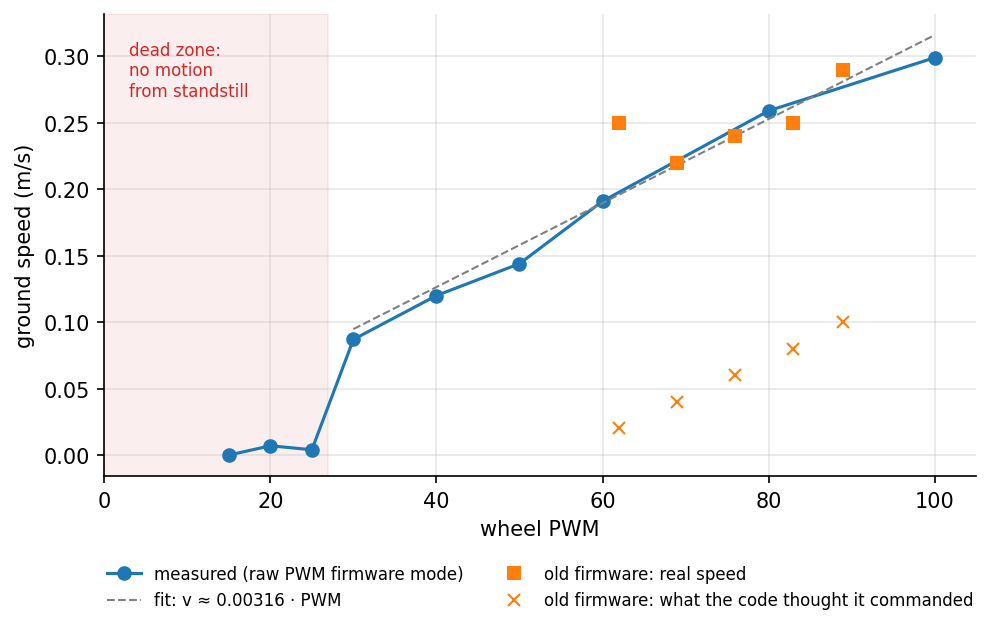
Driving straight at a wall at constant command, the ultrasonic range $d(t)$ decreases linearly and the ground speed is the slope of a least-squares fit, $\hat v = -\,\mathrm{d}d/\mathrm{d}t$, taken after the initial transient. The same data give the reaction time, defined as the delay between the command and the extrapolated start of the motion, and the stopping distance. The first run produced 0.29 m/s for a commanded 0.10 m/s. The original firmware added a fixed minimum PWM and assumed a top speed of 0.5 m/s, so every command was roughly three times faster than intended, and the "slow" setting of my first controller was in fact 0.4 m/s.
I added a raw-PWM command mode to the firmware, reusing a reserved byte of the command packet as a mode flag and extending the checksum over it so that existing packets remained valid. With raw PWM the response is close to linear, $v \approx 0.00316\ \text{m/s} \times \text{PWM}$, above a dead zone: from standstill the car does not move at all at PWM 25 or below and reaches normal speed at 30. The reaction time is 150 to 250 ms, most of it transport delay; the fitted motor model itself reaches 63% of its final speed in about 50 ms.
The tape as a protractor
Yaw rate was measured with the line itself. Spinning in place over a straight piece of tape, the IR sensors sweep across it twice per revolution; the interval between sweeps gives the yaw rate directly, without a gyroscope. For a differential-drive vehicle with track width $B$ the no-slip yaw rate is $\omega_0 = (v_R - v_L)/B$. The measured ratio $\eta = \omega/\omega_0$ was only 0.26 to 0.34 across PWM 45 to 80, and spinning stalled almost completely at PWM 30.
The explanation is skid-steer kinematics. With four wheels rigidly aligned, the car can only rotate if its tyres slide sideways about the instantaneous centre of rotation, and the friction from that scrubbing absorbs most of the torque. Equivalently, the vehicle behaves like an ideal differential drive with an effective track width $B/\eta$, roughly three times its physical width. How much scrubbing the tyres do depends on the ratio of axle spacing to track width, which turned out to be the most important number in the whole model.
A labelling error that looked like physics
Before any of this, the hand-written controller drove the car in circles. Tuning did not help, because the cause was not dynamic: on this car the analog input I had labelled "left" is wired to the right sensor, so every correction steered away from the line. A static test with the tape under one side of the car settled it in seconds. I had earlier concluded the opposite from a photograph in which the tape was only a few millimetres off centre, which is a reminder that a confident conclusion from marginal evidence is worse than no conclusion.
Geometry from the manufacturer's CAD
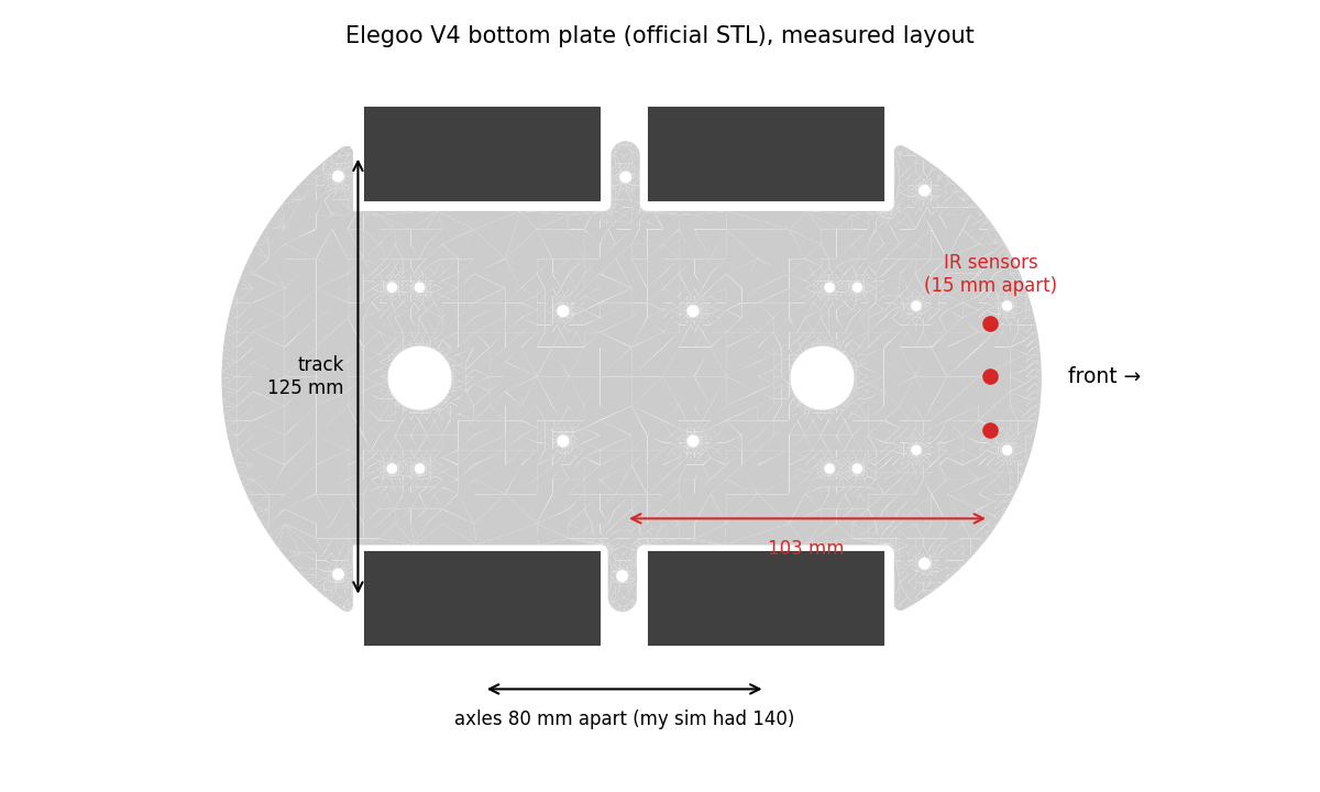
My first model used dimensions estimated by eye. Elegoo publishes the acrylic chassis plates as STL files, so I parsed them directly, rendered the top surface and measured the wheel cut-outs and mounting holes. The real axles are 80 mm apart and the wheels 125 mm apart, against 140 mm and 145 mm in my model; the IR sensors sit about 103 mm ahead of the centre between the axles. The ratio that governs skid-steer turning was 0.97 in the model and is about 0.64 on the car, so the real vehicle turns considerably more easily than the one I had been training on.
Fitting the drivetrain
In MuJoCo each wheel is driven by a velocity actuator. With a physically realistic gain, that actuator is a
first-order DC motor model, with the PWM duty cycle $d$ as input:
Motor model
$$\tau = k_v\,\bigl(\omega_{\text{nl}}\, d - \omega\bigr), \qquad d = \frac{\text{PWM}}{255}, \qquad \tau_{\text{stall}} = k_v\,\omega_{\text{nl}}.$$The three free parameters, motor gain $k_v$, no-load speed $\omega_{\text{nl}}$ and tyre friction $\mu$, are fitted by minimising the relative error against the measured straight-line speeds $v_i$ and spin rates $\omega_j$,
$$\phi^\star = \arg\min_{\phi = (k_v, \omega_{\text{nl}}, \mu)}\ \sum_i \Bigl(\frac{\hat v_i(\phi) - v_i}{v_i}\Bigr)^2 + \sum_j \Bigl(\frac{\hat\omega_j(\phi) - \omega_j}{\omega_j}\Bigr)^2,$$where each term requires a short MuJoCo rollout, and the optimisation runs with Nelder–Mead in log-parameter space. With the estimated geometry, the fit converged to a stall torque of 1.1 N·m per wheel, several times what a TT gear motor can deliver: the optimiser was compensating for the wrong shape with an impossible motor. With the geometry from the STL files the same fit gives 0.23 N·m, a plausible value, and matches straight-line speeds within about 10% and spin rates within 10 to 27%. A physically sensible parameter falling out of a fit is a useful check that the model structure is right.
The simulator
Sensors and communication
Each IR sensor is modelled as a circular spot of radius $r$ at lateral distance $d$ from the tape centreline. The covered fraction of a disc against a strip of half-width $h$ has a closed form. Let $A(y) = r^2 \arccos(-y/r) + y\sqrt{r^2 - y^2}$ be the area of the disc lying below a chord at height $y \in [-r, r]$. Then
$$c(d) = \frac{A(h - d) - A(-h - d)}{\pi r^2}, \qquad a = \operatorname{clip}\bigl(g\, c(d) + b + |n_{\text{grain}}| + \varepsilon,\ 0,\ 1\bigr),$$with a per-sensor gain $g$, a floor offset $b$, slowly varying grain noise $n_{\text{grain}}$ modelled as an Ornstein–Uhlenbeck process, and white noise $\varepsilon$. The gain range of 1.1 to 2.6 reproduces a property found in a static test: with the tape centred between two sensors, both read close to full scale, so the real sensors saturate at roughly half coverage. The floor offset range of up to 0.35 comes from real readings over bare laminate, where the centre sensor averaged 0.25.
The radio link is modelled as a transport delay of $k$ control steps together with dropped commands. BLE writes on this module require an acknowledgement of about 66 ms, so the control loop skips a write while the previous one is still in flight. In the simulator, the command that reaches the motors is
$$\tilde{\mathbf u}_t = \begin{cases} \mathbf u_{t-k} & \text{with probability } 1 - p_{\text{drop}} \\ \tilde{\mathbf u}_{t-1} & \text{otherwise,} \end{cases} \qquad k \in \{3, \dots, 6\}\ (150\text{–}300\ \text{ms}),\quad p_{\text{drop}} \in [0, 0.35].$$The ultrasonic sensor is three MuJoCo rangefinder rays spanning the HC-SR04's beam, including its habit of returning "no echo" for objects closer than about 10 cm. Obstacles are mocap boxes repositioned each episode, so the scene never needs to be recompiled.
Domain randomisation and curriculum
| Parameter | Distribution at full difficulty | Basis |
|---|---|---|
| Transport delay | 3–6 steps (150–300 ms) | Wall-test reaction time |
| Dropped commands | $p_{\text{drop}} \sim U(0, 0.35)$ | BLE acknowledgement time |
| Motor dead zone | PWM 22–30 | Low-PWM wall test |
| Motor gain, left/right mismatch | $\times U(0.8, 1.2)$, $\times U(0.92, 1.08)$ | Around the fit |
| Tyre friction, chassis mass | $\times U(0.75, 1.25)$, $\times U(0.85, 1.2)$ | Around the fit |
| Tape width, sensor spacing | 14–16 mm, 14–16 mm | Measured |
| Sensor position ahead of centre | 93–113 mm | Plate STL |
| IR gain, floor offset, grain | 1.1–2.6, −0.03–0.35, $\sigma \le 0.15$ | Static tests, floor readings |
Training courses are procedurally generated: closed loops driven in either direction and open paths with sharp or filleted turns. A difficulty level $\lambda \in [0.2, 1]$ grows linearly over the first 60% of training, $\lambda(t) = 0.2 + 0.8\,\min(1, t/0.6T)$, and scales the scenario distribution: the maximum turn angle ($120° + 50°\lambda$), the probability of junctions, crossings and gaps, the probability of a box on the line ($0.5\lambda$), battery sag, Bluetooth stalls and lateral pushes, as well as the delay, drop and sensor-offset ranges above. The car's ultrasonic emergency stop runs inside the simulator exactly where it runs on the laptop, between the policy output and the radio, so the policy is trained with the same safety layer it is deployed with.
Learning: PPO with an asymmetric critic
The policy is trained with Proximal Policy Optimization. For a batch of trajectories collected by the previous policy, PPO maximises the clipped surrogate objective
$$L^{\text{CLIP}}(\vartheta) = \mathbb{E}_t\Bigl[\min\bigl(\rho_t\,\hat A_t,\ \operatorname{clip}(\rho_t,\, 1-\epsilon,\, 1+\epsilon)\,\hat A_t\bigr)\Bigr], \qquad \rho_t = \frac{\pi_\vartheta(\mathbf u_t \mid \mathbf o_t)}{\pi_{\vartheta_{\text{old}}}(\mathbf u_t \mid \mathbf o_t)},$$with advantages from generalised advantage estimation,
$$\hat A_t = \sum_{l \ge 0} (\gamma\lambda_{\text{GAE}})^l\, \delta_{t+l}, \qquad \delta_t = r_t + \gamma V_\varphi(\mathbf x_{t+1}) - V_\varphi(\mathbf x_t).$$The quality of $\hat A_t$ depends entirely on the critic $V_\varphi$, and a critic that sees only three IR readings has a hard job: the same sensor history can come from a car about to recover or one about to leave the line. Because the critic is only needed during training, it can be given information the robot will never have. This is the asymmetric actor-critic of Pinto et al. The input to both networks is $\mathbf x_t = [\mathbf o_t;\ \mathbf s^{\text{priv}}_t]$, where the privileged part contains the true lateral error and heading, the track curvature 0.1 to 0.3 m ahead, the distance to the next obstacle, the true speed and yaw rate, and the sampled physics parameters. The actor sees a masked copy,
$$\pi_\vartheta(\mathbf u \mid \mathbf m \odot \mathbf x), \qquad V_\varphi(\mathbf x), \qquad \mathbf m = [\,\mathbf 1_{\dim \mathbf o};\ \mathbf 0_{\dim \mathbf s^{\text{priv}}}\,],$$so on the car the privileged part is filled with zeros and the actor is unaffected. In Stable-Baselines3 this amounts to a policy subclass that replaces the actor's feature extractor with the mask; both extractors keep the same output width, so a single MLP head serves both networks.
| Setting | Value |
|---|---|
| Parallel environments, rollout length | 12, 2048 steps each |
| Minibatch, epochs per update | 4096, 5 |
| Discount $\gamma$, GAE $\lambda$ | 0.995, 0.95 |
| Learning rate | $3\cdot10^{-4}$ decaying linearly to $3\cdot10^{-5}$ |
| Clip $\epsilon$, target KL, entropy coefficient | 0.15, 0.03, 0.001 |
| Networks, initial log-std | MLP 256×256, −0.5 |
| Training budget | 20 M steps, about 50 minutes on an M4 Pro |
These settings came from a run whose evaluation return oscillated between 5 and 49 without trending: larger rollouts, a decaying step size and a KL limit stabilised it.
Memory: a frame stack against an LSTM
The observation is not Markov. Three IR readings cannot say which side the line left on once it is out of view, and with a transport delay of 150 to 300 ms the current reading reflects commands sent several steps earlier. The policy therefore needs memory, and there are two standard ways to provide it. The default above is a fixed window: the last eight frames, 0.4 s of history, fed to an MLP. The alternative is a recurrent policy that carries a learned summary of the entire episode,
$$\mathbf h_t = \operatorname{LSTM}\bigl(\mathbf h_{t-1},\ \mathbf m \odot \mathbf x_t\bigr), \qquad \mathbf u_t \sim \pi_\vartheta(\,\cdot \mid \mathbf h_t), \qquad V_\varphi\bigl(\mathbf h^{V}_t\bigr),\quad \mathbf h^{V}_t = \operatorname{LSTM}_V\bigl(\mathbf h^{V}_{t-1},\ \mathbf x_t\bigr).$$
I implemented it with RecurrentPPO from sb3-contrib, using separate actor and critic LSTMs of 128 units with a
128-unit head, and the same asymmetric masking: the actor's LSTM receives the masked input, the critic's receives
everything. PPO then trains on sequences rather than independent samples. Each environment's rollout is cut into chunks of
512 steps, gradients are back-propagated through time within a chunk, and the hidden state is reset at episode boundaries.
On the car the controller carries $\mathbf h_t$ from one control step to the next and resets it at the start of a run.
The cost is speed: sequential backpropagation through the LSTM ran at about 1,100 environment steps per second against
roughly 7,000 for the MLP, so 10 M steps took two and a half hours.
| Simulator of the time, $P = 5$ | L track: finished | Lost the line | Speed |
|---|---|---|---|
| PD controller | 77% | 23% | 0.087 m/s |
| Tuned PPO, 8-frame MLP | 40% | 60% | 0.131 m/s |
| Recurrent PPO, LSTM | 77% | 23% | 0.159 m/s |
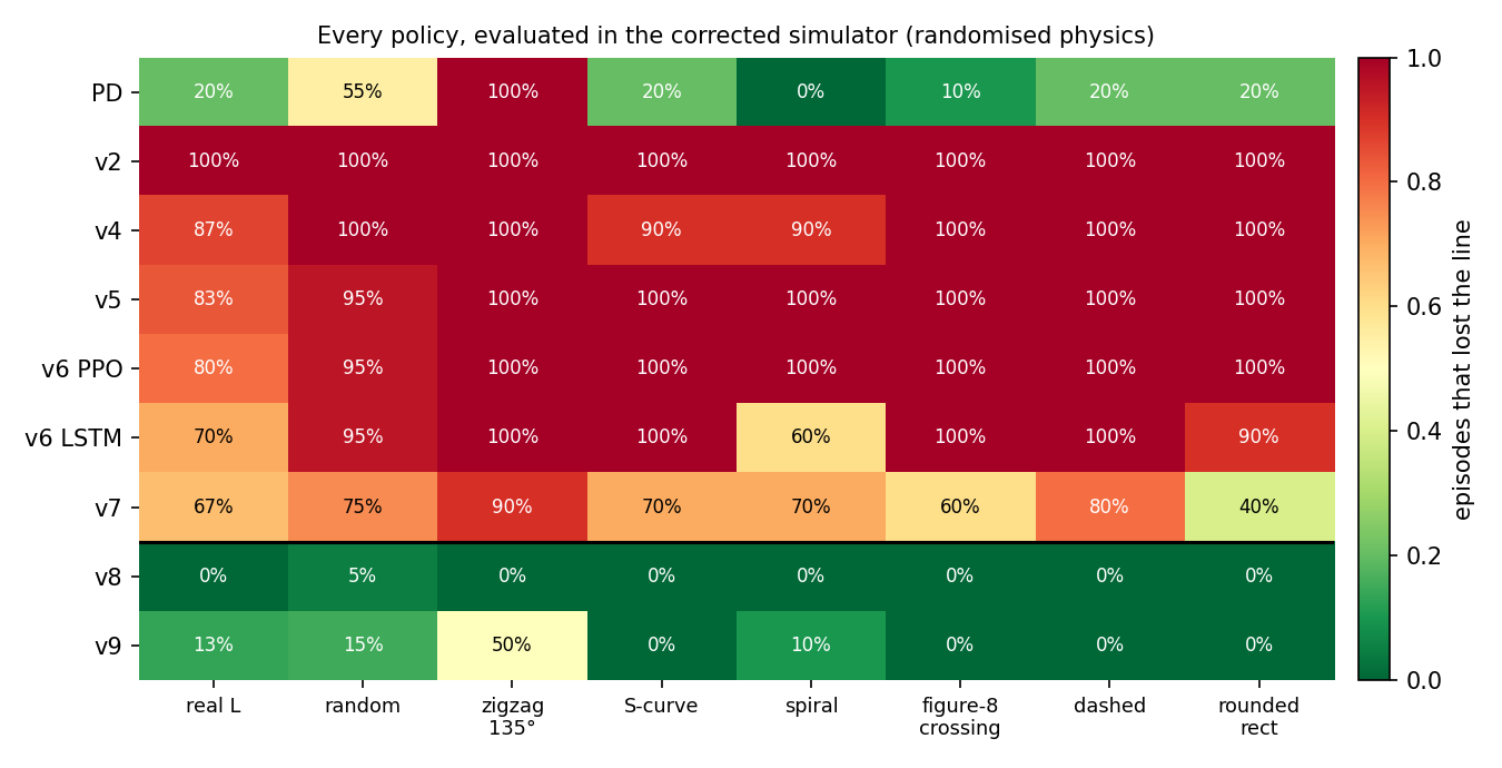
Memory helped. With the same reward the LSTM matched the PD controller's reliability on the L track at nearly twice its speed, where the frame-stack policy lost the line in most runs. It did not change the underlying behaviour, though: on the held-out courses it still lost the line in 30 to 90% of episodes, and in the corrected simulator it fails almost as badly as the other policies of its generation (89% of episodes lost, against 96 to 97% for the MLPs). The limiting factor was the reward, which is the subject of the next section, and the LSTM was trained before that was fixed. A recurrent policy trained with the corrected reward in the corrected simulator is the obvious experiment I have not yet run.
The reward, and the price of a failure
The per-step reward pays for progress along the line, discounted by distance from it, and penalises abrupt action changes. Leaving the line or hitting an obstacle ends the episode with a penalty $P$:
$$r_t = 20\,\Delta s_t\,\max\!\Bigl(0,\ 1 - \frac{|e_t|}{30\ \text{mm}}\Bigr) - 0.05\,\bigl\|\mathbf u_t - \mathbf u_{t-1}\bigr\|^2 - P\,\mathbb 1[\text{lost or collided}].$$Every policy trained with $P = 5$, whether plain PPO, tuned PPO or the LSTM, converged to the same behaviour: twice as fast as the hand-written controller and noticeably less reliable. The reason is visible in the expected return. Ignoring discounting, $J(\pi) \approx 20\,\mathbb E[S] - P\,\Pr(\text{fail})$, where $S$ is the distance covered, so a change to the policy improves the objective whenever
$$20\,\Delta\mathbb E[S] > P\,\Delta\Pr(\text{fail}).$$With $P = 5$, a one-percentage-point increase in failure risk is repaid by just 2.5 mm of extra expected progress, so the optimiser was right to trade reliability for speed. With $P = 40$ the same risk costs 2 cm, and the optimum moves. In the simulator of the time, tuned PPO trained with $P = 40$ completed 97% of L-track runs, against 40% for the same algorithm with $P = 5$ and 77% for the LSTM. No change of algorithm had moved the number that far.
Validating the simulator by predicting failures
Two policies failed on the real car in instructive ways. Version 2 oscillated at full steering from the first second. The logs showed four discrepancies that the simulator did not reproduce: the centre sensor read 0.25 over bare floor where the model allowed at most 0.08, the delay was longer and a quarter of the commands were dropped, nothing in the reward discouraged bang-bang steering, and the speed cap used on the car was absent in training. To the policy, a reading of 0.25 meant "the edge of the tape is under me", so it corrected towards a line that was not there, a quarter of a second late. Once those effects were added, the simulator reproduced the failure: the same policy completed the track in only 10% of simulated runs.
Version 7, trained with the corrected reward, weaved across the tape about three times a second on the real car and lost it after six seconds, despite completing 97% of simulated runs. This time no single parameter in the simulator could reproduce the run. The missing pieces were the measured dead zone, the measured tape and sensor geometry, the saturating sensor response and, above all, the vehicle geometry from the STL files. After those corrections the simulator predicted v7's failure: 37% completions and 63% lost runs.
That became the acceptance test for every subsequent change. A simulator that agrees with a policy you hope will work tells you very little; one that correctly predicts a failure you have already observed is worth training on. Re-evaluating every policy version in the corrected simulator, on the real track and seven other courses under randomised physics, gives the whole history at a glance:
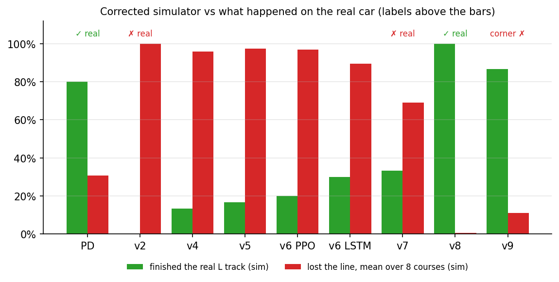
| Version | What changed | Real car |
|---|---|---|
| v1 | First sim-to-real environment; the track generator produced only left turns | not tested |
| v2 | Balanced tracks; beat the PD controller in the original simulator | oscillated, lost the line at 2.5 s |
| v3 | Measured floor offsets, delay and drops added all at once; did not learn | not tested |
| v4–v6 | Curriculum, scenarios, ultrasonic, privileged critic, safety layer in training, tuned PPO and LSTM | not tested |
| v7 | Failure penalty 5 → 40 | weaved, lost the line at 6 s |
| v8 | Corrected geometry, dead zone, tape and sensor geometry, saturating IR | drove the full track |
| v9 | v8 plus dead-zone compensation | smoother straight, failed at the corner |
The first policy that drove the real track
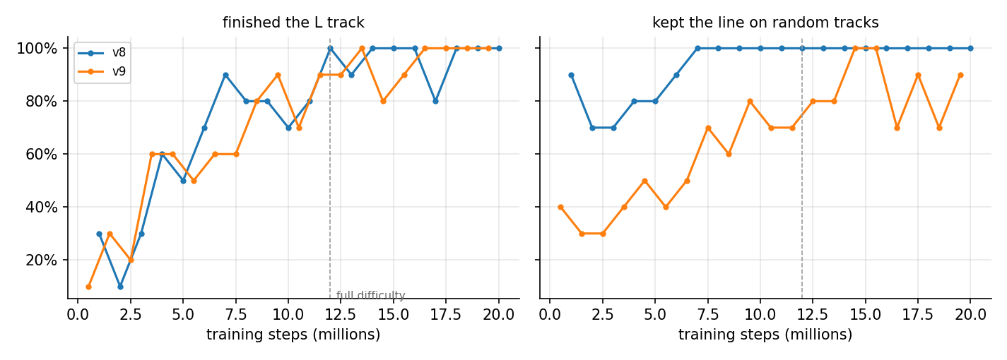
In the corrected simulator v8 completed the L track in all 30 randomised runs and lost the line in 1% of episodes across the eight courses. How it achieved that is as interesting as the result. Only 4 to 12% of its wheel commands fell inside the dead zone, against 24% for v7 on the real car: it had learned to keep both wheels turning rather than stopping the inner wheel to steer. On the floor, against the hand-written controller and the previous version:
| Real car, L track | PD controller | v7 | v8 |
|---|---|---|---|
| Frames with the tape under a sensor | 92% | 27% | 92% |
| Longest interval without the tape | 0.7 s | 13.6 s | 0.7 s |
| Frames with the centre sensor on the tape | 56% | 14% | 63% |
| Left/right sensor swaps per second | 1.7 | – | 2.3 |
| Corner | completed | not reached | completed |
| Speed on the straight | 0.078 m/s | – | 0.073 m/s |
The result matches the hand-written controller on keeping the tape in view and keeps the centre sensor on it more often, from a policy that had never interacted with the real car. It also wobbles more, which is the subject of the final part of this article. Beyond the real track, the same weights handle courses that do not appear in training:
Hairpins remain the open case. On a zigzag with 135° turns the hand-written controller loses the line in every episode; v8 never loses it, but it did not complete the course in any of ten runs, creeping into the first hairpin and stalling there.
Why it still wobbles
Turning with one wheel stopped
A final open-loop test isolated the remaining discrepancy. Holding the left side at PWM 45 with the right side stopped, the real car turns half a circle in six seconds, about 0.52 rad/s; the simulator predicts 0.07 rad/s. With both sides moving, at PWM 45 and 30, simulator and car agree to within a few degrees over six seconds. The model is accurate in one regime and wrong by a factor of eight in another, and the dead zone pushes the controller into the wrong one: any small correction that commands the inner wheel below about PWM 27 stops it dead, and the real car then turns far harder than the policy expects. Adding a separate braking coefficient for a stopped wheel to the fit made the prediction worse, so this is a limitation of the model structure rather than of its parameters.
The pragmatic response is to keep the car out of that regime. Version 9 adds dead-zone compensation, mapping every non-zero command to at least PWM 28 in the simulator and on the car alike, so that a correcting wheel slows down instead of stopping. On the real car this cut the fraction of time with one side stopped from 48% to 17% and the rate of left/right sensor swaps from 2.3 to 1.0 per second, and the car drove the straight at 0.16 m/s, twice as fast as v8. It then overshot the corner, reversed, spun and lost the line, which the logs alone could not explain.
Ground truth from a phone video
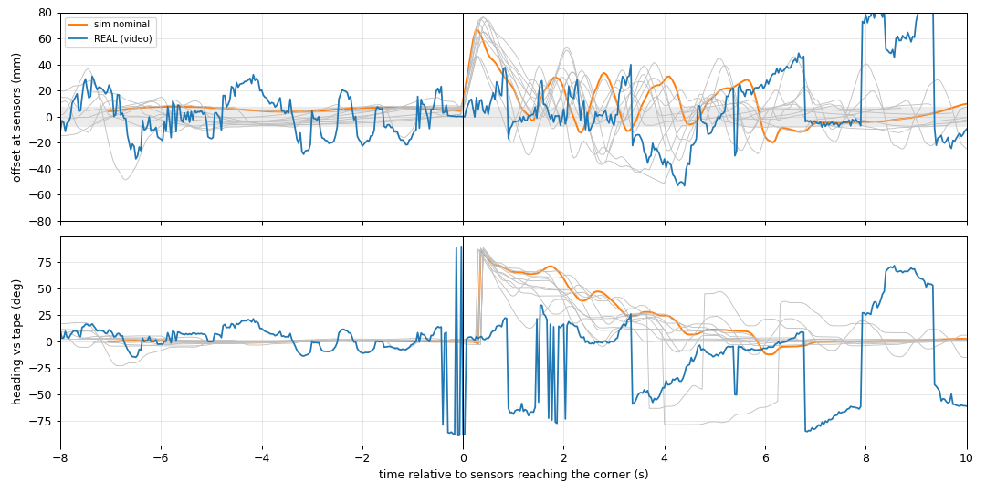
The car's logs record what its sensors saw, not where it was. To recover the latter I filmed a run with a hand-held phone and wrote a tracker that measures everything in the car's own frame, which makes camera motion irrelevant. In each frame the car is the largest connected region that is not floor (dark, saturated or very bright pixels, closed and opened morphologically to remove the thin tape), and its minimum-area rectangle gives the position $\mathbf c$, heading $\hat{\mathbf a}$ and scale from the 231 mm plate length. The remaining dark pixels are the tape, fitted with up to two lines $(\mathbf p, \hat{\mathbf d})$ by RANSAC. With the sensor point $\mathbf s = \mathbf c + 103\ \text{mm}\cdot\hat{\mathbf a}$ and the car's lateral axis $\hat{\boldsymbol\ell}$, the measured lateral offset and heading error are
$$e = \bigl(\mathbf p + \hat{\mathbf d}\,\hat{\mathbf d}^{\!\top}(\mathbf s - \mathbf p) - \mathbf s\bigr)\cdot\hat{\boldsymbol\ell}, \qquad \psi = \operatorname{atan2}\bigl(\hat{\mathbf d}\cdot\hat{\boldsymbol\ell},\ \hat{\mathbf d}\cdot\hat{\mathbf a}\bigr),$$and where two legs are visible, their intersection locates the corner in the car frame. The video is aligned with the log by the lag that maximises the correlation between the video offset and the IR centroid, $\delta^\star = \arg\max_\delta \operatorname{corr}\bigl(e_{\text{video}}(t+\delta),\, e_{\text{IR}}(t)\bigr)$, which places the start of the run exactly where the video shows the car begin to move.

| v9, real track | Offset std (straight) | Heading std (straight) | Weave period | Max overshoot, first 4 s at the corner |
|---|---|---|---|---|
| Real car (video) | 15.6 mm | 8.8° | ~1.0 s | 102 mm |
| Simulator, nominal parameters | 1.3 mm | 0.4° | ~4 s | 66 mm |
| Simulator, randomised (10 runs) | 7.0 mm | 3.2° | ~6 s | 65 mm |
Separating the vehicle from the sensors
To determine whether the discrepancy lies in the vehicle model or the sensor model, I replayed the exact wheel commands from the real log into the simulated car, open loop, with neither the policy nor the sensors involved, and compared the resulting heading with the video. The real heading spans 36° over the straight; the simulated car, driven by identical commands, spans 17°. The best timing agreement occurs with a command-to-motion delay of about 100 ms, shorter than the 150 to 300 ms used in training, and the largest errors occur at higher speed when the left wheels run faster than the right. That is consistent with the slight rightward drift visible in the very first wall tests, and it identifies a gap in the randomisation: I randomised left/right torque, which barely affects free-running speed, but never left/right speed, which is what makes a car drift. A grid search over a left/right speed ratio, a friction scale and the delay reduces the heading error of the replay from 10.4° to 8.2° RMS, with a left side 10 to 30% faster, friction scaled by 0.5 to 0.7 and a delay of 50 to 100 ms, but it explains only part of the difference.
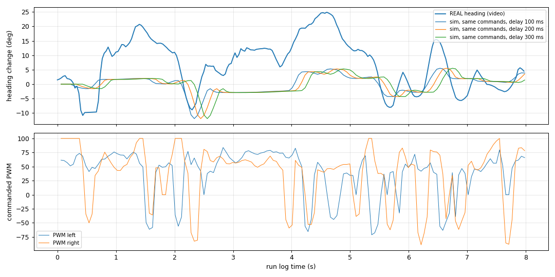
Why the weave has a one-second period
The period of the oscillation is itself informative. Near the line, the heading loop is approximately an integrator, since heading is the integral of yaw rate, preceded by the loop delay $\tau$. The open-loop transfer function of a proportional correction with gain $K$ is then
$$L(s) = \frac{K\, e^{-s\tau}}{s}, \qquad \angle L(j\omega) = -\frac{\pi}{2} - \omega\tau.$$The phase reaches $-\pi$ at $\omega_{180} = \pi/(2\tau)$, so the loop is stable only for $K < \pi/(2\tau)$, and when that margin is exceeded it oscillates with period
$$T_{\text{osc}} = \frac{2\pi}{\omega_{180}} = 4\tau.$$With an end-to-end loop delay of 0.2 to 0.25 s, the reaction time measured on the wall test and made up of sensor sampling at 25 Hz, the control period and the acknowledged radio write, this predicts a weave period of 0.8 to 1.0 s. The video measured 1.0 s. The replay supplies the other half of the explanation: the policy's corrections were tuned on a vehicle whose yaw response is roughly half as strong as the real one, so on the real car the effective gain sits above the stability margin. The policy is not noisy. It is a reasonable controller operating a plant that is more responsive than the one it was trained on.
Discussion and next steps
Most of the progress in this project came from measurement rather than learning. The geometry error cost more than any choice of algorithm or hyperparameter, and the manufacturer had published the correct numbers all along. The reward error affected every algorithm equally, because each one optimised the objective it was given. The labelling errors (a swapped pair of sensor inputs, a track generator that produced only left turns, a one-count noise spike that flipped a search direction) produced symptoms that looked like dynamics and would not have been found by tuning. The most useful methodological habit was to treat the simulator as a model under test, and to accept a change only when it made the simulator predict what the real car had already done.
The evidence has limits that are worth stating. The real-car results come from a single track and a handful of runs per policy, the simulated evaluations use 10 to 30 episodes per condition, and the video comes from a hand-held camera, which adds a few degrees of noise to every heading measurement. The conclusions are robust to those limits because the effects are large, but the exact percentages should be read as estimates.
The next iteration follows directly from the replay. Left/right speed asymmetry will be measured with straight-line runs at PWM 70 and 100 and added to both the model and the randomisation, the turning model will be refitted with the replay error as its objective, and the delay range will be centred on 50 to 200 ms. The turning response will then be randomised over a range wide enough to contain the measured factor of two, so that the policy learns to be stable across it, and the result will be judged by the same video comparison, ideally with a recurrent policy as well as the frame stack, since the oscillation is exactly the kind of history-dependent effect memory can compensate for. After that come real courses beyond the L track, and eventually the ESP32 camera, starting from line features extracted from the image rather than raw pixels.
Code
The project is organised so that every experiment above is a single command.
mjsim/
  elegoo_v4.xml         MuJoCo model, geometry from the official plate STLs
  calibrate.py          fits motor gain, no-load speed and friction to the measurements
  car_env.py            sim-to-real environment: sensor and link models, randomisation, curriculum
  baseline.py           the real-car PD controller inside the simulator
  watch_training.py     drives the newest checkpoint next to the learning curves while training
  export_blender.py     records a run; blender_scene.py renders it in Blender
rl/
  train_car.py          PPO, tuned PPO and LSTM training; regression suite on held-out courses
  privileged.py         asymmetric actor-critic for Stable-Baselines3
hardware/
  wall_test.py          ultrasonic speedometer
  turn_test.py          yaw rate from tape crossings
  circle_test.py        fixed PWM pairs, with the simulator's prediction via --sim
  video_track.py        car-frame tracking from a phone video, synchronised to the run log
# train, evaluate on held-out courses, deploy without fine-tuning
python3 -m rl.train_car --config v9 --algo ppo_tuned --steps 20000000 --out rl/policy/v9_ppo
python3 -m rl.train_car --suite rl/policy/v9_ppo/car_ppo.zip
python3 -m hardware.run_hardware --link ble --controller car_rl --model rl/policy/v8_ppo/car_ppo.zipThe full project is at github.com/airo7/sim2real-robot-car.
References
- Todorov, Erez & Tassa (2012). MuJoCo: A physics engine for model-based control. IROS.
- Schulman et al. (2015). High-Dimensional Continuous Control Using Generalized Advantage Estimation. arXiv:1506.02438.
- Schulman et al. (2017). Proximal Policy Optimization Algorithms. arXiv:1707.06347.
- Tobin et al. (2017). Domain Randomization for Transferring Deep Neural Networks from Simulation to the Real World. IROS.
- Peng et al. (2018). Sim-to-Real Transfer of Robotic Control with Dynamics Randomization. ICRA.
- Pinto et al. (2018). Asymmetric Actor Critic for Image-Based Robot Learning. RSS.
- Raffin et al. (2021). Stable-Baselines3: Reliable Reinforcement Learning Implementations. JMLR 22(268).
- ELEGOO Smart Robot Car Kit V4.0, official repository including the chassis STL files: github.com/elegooofficial/ELEGOO-Smart-Robot-Car-Kit-V4.0.
- Part 1: Reinforcement Learning vs Model Predictive Control.
- Part 2: MPC vs RL on the Cart-Pole: An Implementation Study.